Building a random network from scratch — a tour of `Network`’s conventions

Every preset in g2elin_core.network.presets is hand-transcribed from a MATLAB source and satisfies the schema’s structural conventions by construction. This notebook goes the other way: it builds a Network programmatically, from a random topology, using nothing but the raw schema types (Bus, Line, Transformer, Load, DerUnit) — the same building blocks the web UI’s drag-and-drop canvas builder uses, and the same building blocks any script that generates test cases would use.

The point isn’t the random network itself (it’s a throwaway topology, not a physically meaningful case study) — it’s the process of building one correctly, and what happens when you don’t. Two validation layers are exercised along the way:

Network’s own pydantic validators — enforced unconditionally, every time a Network is constructed: every bus reference must resolve, and there must be exactly one slack DER unit. You cannot construct an instance that violates these; the exception happens at Network(...) itself.
network.validation.validate_network() — a further, opt-in check for everything syntactically valid but still structurally wrong: a DER not sitting behind its own transformer, a line or load landing directly on a DER’s private bus, a disconnected network, and so on. These are easy to produce by construction (especially programmatically or via drag-and-drop) and would otherwise surface as a bare crash deep inside power flow, modal analysis, or EMT — see docs/sphinx/modules/network.md’s “Validation” section for the full account of why this module exists.

We’ll build one clean random network the right way, run the full analysis pipeline on it, then deliberately break several copies of it to see exactly what each validation layer catches — and close with a batch of many random networks to show the builder is robust across sizes and seeds, not just one lucky draw.

%matplotlib inline
import math

import numpy as np
import pandas as pd
import matplotlib.pyplot as plt
import networkx as nx

plt.rcParams["figure.dpi"] = 100
pd.set_option("display.precision", 4)
np.set_printoptions(precision=4, suppress=True)

from g2elin_core.network.schema import (
    Bus, Line, Transformer, Load, DerUnit, Network, BusType, UnitType, GfmController,
)
from g2elin_core.network.validation import validate_network
from g2elin_core.network.topology import compute_topology_layout
from g2elin_core.powerflow import run_power_flow
from g2elin_core.pipeline import linearize_network
from g2elin_core.modal import analyze

RNG_SEED = 42

Run-time toggles

Section 6 (nonlinear EMT simulation) is one of the slowest cells in this notebook – a full nonlinear coupled-Newton time integration, not just linear algebra. Defaults to off so “Restart Kernel and Run All” finishes quickly; flip the flag to True and re-run to actually exercise that section.

RUN_EMT_SECTION = True  # Section 6: nonlinear EMT time-domain simulation

1. The convention a network builder has to respect

Paraphrasing network.md’s Validation section, and matching Functions/network_form.m’s original MATLAB convention:

Every DER unit (sm/gfm/gfl/infinite_bus) sits on its own private bus, reached from the rest of the network through exactly one transformer — never a Line, never shared with another DER, never another transformer’s hv_bus.
A DER’s own local consumption is its p_cons_mw/q_cons_mvar fields, not a separate Load on its private bus.
Exactly one DER unit has bus_type = slack, and for modal analysis/EMT to work it should be an sm or infinite_bus (a gfm/gfl slack is accepted for power flow but not wired into interconnect.network_assembly yet — validate_network() flags this as a warning, not an error).
The whole graph (buses + lines + transformers) must be connected — every bus must be reachable from the slack.

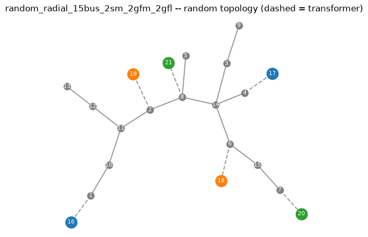
None of that is specific to any one topology shape — a schema-valid network can be meshed or radial, tiny or large, one DER or twenty. The builder below picks a specific, deliberately realistic shape on top of those rules: a radial (tree — no loops) feeder of at least 15 buses, carrying exactly 2 SM + 2 GFM + 2 GFL, each tapping a different point on the feeder (no two DERs ever share a connection point) — the kind of topology and DER mix an actual distribution-feeder hosting- capacity study would look at, not just the smallest schema-valid example. Every rule above is still enforced explicitly, with a comment at each step naming which one.

def random_network(
    rng: np.random.Generator,
    n_grid_buses: int = 15,
    load_fraction: float = 0.6,
    sn_mva: float = 100.0,
    f_hz: float = 60.0,
    hv_kv: float = 230.0,
    lv_kv: float = 18.0,
    name: str | None = None,
) -> Network:
    '''A random, but *convention-respecting*, network: a random RADIAL
    (tree-topology -- no loops) grid at ``hv_kv`` with at least 15 buses,
    random loads on a subset of them, and exactly 2 SM + 2 GFM + 2 GFL
    DER units (the first SM forced to the slack) each on its own new bus
    at ``lv_kv``, reached by its own transformer -- and each connected to
    a *different* grid bus, so no two DERs ever share a connection point.
    '''
    if n_grid_buses < 15:
        raise ValueError(f"n_grid_buses must be >= 15 (need room for 6 non-colliding DER taps), got {n_grid_buses}")

    grid_bus_ids = list(range(1, n_grid_buses + 1))
    buses = [Bus(id=i, name=f"bus{i}", vn_kv=hv_kv) for i in grid_bus_ids]

    # Radial rule: the grid topology *is* a random spanning tree, full
    # stop -- nothing added on top. A tree has exactly n-1 edges and, by
    # construction, no cycles, which is exactly what "radial" means for a
    # feeder (as opposed to a meshed transmission network) -- and it
    # still guarantees every bus is reachable from every other one, the
    # same connectivity rule a meshed topology would also have to satisfy.
    tree_seed = int(rng.integers(0, 2**31 - 1))
    tree = nx.random_labeled_tree(n_grid_buses, seed=tree_seed)
    edges = sorted((min(u, v) + 1, max(u, v) + 1) for u, v in tree.edges())

    # Distribution-feeder-scale impedance (matching CIGRE_raw.m's own
    # per-line r_pu/x_pu order of magnitude), not the WSCC-style
    # transmission-line values an earlier version of this builder used --
    # those were tuned for a handful of buses with redundant paths; a
    # purely radial chain of 15+ buses has no redundant path to share
    # current with, so a single hop's impedance accumulates all the way
    # down the tree. At transmission-line scale that accumulation
    # regularly pushed power flow to non-convergence on the larger/longer
    # trees this builder can now draw; at this scale it didn't, across 50
    # test seeds (see the notebook's own Section 10 for the same claim
    # exercised in-line, not just asserted here).
    lines = [
        Line(
            from_bus=u, to_bus=v,
            r_pu=round(float(rng.uniform(0.001, 0.008)), 4),
            x_pu=round(float(rng.uniform(0.003, 0.02)), 4),
            b_pu=round(float(rng.uniform(0.001, 0.02)), 4),
            length_km=round(float(rng.uniform(1.0, 20.0)), 1),
            name=f"line_{u}_{v}",
        )
        for u, v in edges
    ]

    # Exactly 2 SM + 2 GFM + 2 GFL, in this fixed order -- der id 1 is
    # always the slack SM (a supported slack type; see
    # validate_network()'s own warning for what happens if a GFM/GFL ends
    # up there instead).
    der_spec = [
        (UnitType.SYNCHRONOUS_MACHINE, BusType.SLACK),
        (UnitType.SYNCHRONOUS_MACHINE, BusType.PV),
        (UnitType.GFM, BusType.PV),
        (UnitType.GFM, BusType.PV),
        (UnitType.GFL, BusType.PQ),
        (UnitType.GFL, BusType.PQ),
    ]
    n_der = len(der_spec)

    # DER placement: one new private bus + one dedicated transformer per
    # unit, id'd past every grid bus id -- never touched by a Line/Load/
    # another Transformer above. `replace=False` is the "no two DERs
    # connected to the same node" rule -- each of the 6 taps lands on its
    # own distinct grid bus, never two DERs sharing one.
    der_bus_ids = [n_grid_buses + 1 + k for k in range(n_der)]
    der_buses = [Bus(id=b, name=f"der{k + 1}_terminal", vn_kv=lv_kv) for k, b in enumerate(der_bus_ids)]
    dispatch_buses = rng.choice(grid_bus_ids, size=n_der, replace=False)

    der_units: list[DerUnit] = []
    transformers: list[Transformer] = []
    p_set_by_der: list[float] = []
    for k, (der_bus, dispatch_bus, (unit_type, bus_type)) in enumerate(zip(der_bus_ids, dispatch_buses, der_spec)):
        controller = GfmController.DROOP if unit_type == UnitType.GFM else None
        xd_pu = round(float(rng.uniform(0.15, 0.28)), 3) if unit_type == UnitType.SYNCHRONOUS_MACHINE else None
        # Dispatch (P_set) is decided here, before loads, so total load
        # can be sized as a *fraction of total dispatched generation*
        # below -- an arbitrary flat load range would routinely exceed
        # what 6 random DERs can actually supply and leave power flow
        # infeasible, which isn't a schema-convention issue but would
        # make the rest of this notebook's random draws unusable.
        p_set_mw = round(float(rng.uniform(0.5, 1.0) * sn_mva), 1)
        p_set_by_der.append(p_set_mw)

        der_units.append(DerUnit(
            id=k + 1, bus=der_bus, unit_type=unit_type, bus_type=bus_type,
            v_set_pu=round(float(rng.uniform(0.98, 1.03)), 3),
            p_set_mw=p_set_mw,
            q_set_mvar=0.0,
            p_cons_mw=round(0.001 * sn_mva, 3),  # own consumption -- never a separate Load
            controller=controller, xd_pu=xd_pu,
        ))
        transformers.append(Transformer(
            hv_bus=int(dispatch_bus), lv_bus=der_bus,  # -- always dispatch (grid) bus -> DER's own bus
            r_pu=0.0, x_pu=round(float(rng.uniform(0.05, 0.09)), 4),
            sn_mva=sn_mva, name=f"der{k + 1}_xfmr",
        ))

    # Loads only ever reference a *grid* bus -- never a DER's own bus.
    # Sized as a fraction of total dispatched generation (leaving the
    # slack real headroom to balance losses), split across the chosen
    # load buses with a Dirichlet draw so shares vary but always sum to
    # the target total.
    load_bus_ids = [b for b in grid_bus_ids if rng.random() < load_fraction] or [grid_bus_ids[0]]
    # A floor on both P and Q (not just fine rounding) matters once there
    # can be 15+ load buses splitting one Dirichlet draw: a bus landing on
    # a tiny share is real, but a *rounded-to-zero* Q would make that
    # load's equivalent reactance (operating_point.py's load_rx -> Lc in
    # components/load.py) exactly zero -- a division by zero inside the
    # linearizer's Jacobian, surfacing as a cryptic "cannot convert
    # complex to float" (sympy's `zoo` for 1/0) instead of anything about
    # the actual load. A strictly-positive floor makes that categorically
    # impossible rather than merely unlikely.
    total_load_mw = sum(p_set_by_der) * float(rng.uniform(0.5, 0.7))
    shares = rng.dirichlet(np.ones(len(load_bus_ids)))
    loads = [
        Load(
            bus=b,
            p_mw=round(max(total_load_mw * share, 0.05), 4),
            q_mvar=round(max(total_load_mw * share * float(rng.uniform(0.2, 0.35)), 0.01), 4),
            name=f"load_bus{b}",
        )
        for b, share in zip(load_bus_ids, shares)
    ]

    return Network(
        name=name or f"random_radial_{n_grid_buses}bus_2sm_2gfm_2gfl",
        f_hz=f_hz, sn_mva=sn_mva,
        buses=buses + der_buses, lines=lines, transformers=transformers,
        loads=loads, der_units=der_units,
    )

2. Build one, and look at it

Network(...)’s own pydantic validators already ran inside the builder above (bus refs resolve, exactly one slack) – if either had been violated, the exception would already have happened before this cell.

rng = np.random.default_rng(RNG_SEED)
net = random_network(rng)

print(net.name, f"-- {net.f_hz} Hz, {net.sn_mva} MVA base")
print(f"{len(net.buses)} buses, {len(net.lines)} lines, {len(net.transformers)} transformers, "
      f"{len(net.loads)} loads, {len(net.der_units)} DER units")
for der in net.der_units:
    tag = " (SLACK)" if der.bus_type == BusType.SLACK else ""
    print(f"  DER {der.id}: {der.unit_type.value:12s} bus={der.bus:2d} bus_type={der.bus_type.value:5s}"
          f" P_set={der.p_set_mw:7.2f} MW{tag}")

random_radial_15bus_2sm_2gfm_2gfl -- 60.0 Hz, 100.0 MVA base
21 buses, 14 lines, 6 transformers, 11 loads, 6 DER units
  DER 1: sm           bus=16 bus_type=slack P_set=  88.20 MW (SLACK)
  DER 2: sm           bus=17 bus_type=pv    P_set=  65.20 MW
  DER 3: gfm          bus=18 bus_type=pv    P_set=  60.70 MW
  DER 4: gfm          bus=19 bus_type=pv    P_set=  61.70 MW
  DER 5: gfl          bus=20 bus_type=pq    P_set=  64.70 MW
  DER 6: gfl          bus=21 bus_type=pq    P_set=  89.20 MW

3. `validate_network()` — the cheap pre-flight check

This is the same check the web UI’s network editor calls on every edit, and the same one compute_operating_point() runs automatically before doing any real work. On a network built to respect the convention, it comes back clean.

issues = validate_network(net)
print("ok:" , not any(i.severity == "error" for i in issues), " -- ", len(issues), "issue(s)")
for i in issues:
    print(f"  [{i.severity}] {i.message}")

ok: True  --  0 issue(s)

4. Topology, power flow, modal analysis

Exactly the same three calls the tour notebook uses on the hand-written presets – nothing about them is preset-specific, they operate on any Network.

topo = compute_topology_layout(net)

fig, ax = plt.subplots(figsize=(6.5, 5.5))
pos = {n.id: (n.x, n.y) for n in topo.nodes}
for e in topo.edges:
    x1, y1 = pos[e.from_bus]
    x2, y2 = pos[e.to_bus]
    style = "--" if e.kind == "transformer" else "-"
    ax.plot([x1, x2], [y1, y2], style, color="0.6", zorder=1)
colors = {"sm": "tab:blue", "gfm": "tab:orange", "gfl": "tab:green", "infinite_bus": "tab:red", None: "0.5"}
for n in topo.nodes:
    ax.scatter(*pos[n.id], s=260 if n.unit_type else 90, color=colors[n.unit_type], zorder=2)
    ax.annotate(f"{n.id}", pos[n.id], ha="center", va="center", fontsize=8, color="white", zorder=3)
ax.set_title(f"{net.name} -- random topology (dashed = transformer)")
ax.set_axis_off()
plt.show()

../_images/76396f244021cb394b82bb0e250c38097b37d51b90cab8877c4d8c1f266de550.png

pf = run_power_flow(net)
print("converged:", pf.converged, " total losses:", round(pf.total_losses_mw(), 4), "MW")
pf.bus_table().head()

converged: True  total losses: 4.1313 MW

	bus	vm_pu	va_degree	p_net_gen_mw	q_net_gen_mvar
0	1	0.9760	4.7941	-0.0000	-0.0000
1	2	0.9800	7.8786	-7.8553	-2.6346
2	3	0.9765	8.6524	-35.1284	-9.4273
3	4	0.9816	9.8735	-15.7376	-3.6252
4	5	0.9824	8.9588	-0.0000	-0.0000

system = linearize_network(net, pf)
modal = analyze(system.A, system.state_names)
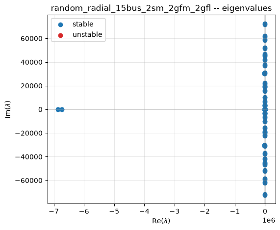
# A strict "< 0" reads as False for *every* network built by this
# codebase, not just this one -- every closed-loop system here has one
# eigenvalue structurally pinned to ~0 (the free reference-angle/"theta
# problem" direction; see docs/sphinx/modules/stability.md), not a real
# instability. A small tolerance separates that from a genuine unstable
# mode.
n_unstable = int(np.sum(modal.eigenvalues.real > 1e-6))
print(f"{system.A.shape[0]} states -- {n_unstable} genuinely unstable mode(s), "
      f"max Re(lambda) = {modal.eigenvalues.real.max():.4f}")

fig, ax = plt.subplots(figsize=(6, 5))
stable = modal.eigenvalues.real < 1e-6
ax.scatter(modal.eigenvalues.real[stable], modal.eigenvalues.imag[stable], color="tab:blue", label="stable")
ax.scatter(modal.eigenvalues.real[~stable], modal.eigenvalues.imag[~stable], color="tab:red", label="unstable")
ax.axvline(0, color="0.3", lw=1)
ax.axhline(0, color="0.85", lw=0.8, zorder=0)
ax.grid(True, alpha=0.3)
ax.set_xlabel(r"Re($\lambda$)"); ax.set_ylabel(r"Im($\lambda$)")
ax.set_title(f"{net.name} -- eigenvalues")
ax.legend()
plt.show()

modal.summary_table().sort_values("undamped_hz").head(10)

176 states -- 0 genuinely unstable mode(s), max Re(lambda) = -0.0000

../_images/2bfec5663f931cb216b53e6e28aae0e9e56b1ba0996b9d7abbf4d05fecaca75c.png

	mode	real	imag	undamped_hz	damped_hz	damping_pct	state1	part1_pct	state2	part2_pct	state3	part3_pct
175	175	-5.4881e-11	0.000	8.7346e-12	0.0000	100.0000	theta_{SM_1}	25.6098	theta_{GFM_2}	25.3387	theta_{SM_2}	24.6553
174	174	-1.8487e-01	0.000	2.9424e-02	0.0000	100.0000	v_pss_{SM_1}	87.8565	v_pss_{SM_2}	11.5185	v_2_{SM_1}	0.1837
173	173	-1.8542e-01	0.000	2.9510e-02	0.0000	100.0000	v_pss_{SM_2}	87.9750	v_pss_{SM_1}	11.4899	v_2_{SM_2}	0.1374
172	172	-4.9832e-01	0.000	7.9310e-02	0.0000	100.0000	v_1_{SM_1}	94.2082	v_1_{SM_2}	3.6103	v_2_{SM_1}	0.9614
171	171	-5.0354e-01	0.000	8.0140e-02	0.0000	100.0000	v_1_{SM_2}	91.4336	v_1_{SM_1}	3.4696	v_2_{SM_2}	1.9056
170	170	-9.9586e-01	0.000	1.5850e-01	0.0000	100.0000	psi_1q_{SM_2}	42.2034	theta_{SM_2}	20.4810	psi_2q_{SM_2}	5.4101
169	169	-1.6056e+00	0.000	2.5554e-01	0.0000	100.0000	psi_1q_{SM_1}	70.7106	theta_{SM_1}	6.6197	psi_2q_{SM_1}	4.8560
160	160	-3.1643e+00	0.000	5.0362e-01	0.0000	100.0000	psi_1q_{SM_2}	27.7581	P_m_{SM_2}	18.6199	P_m_{SM_1}	16.3948
163	163	-2.4422e+00	3.871	7.2845e-01	0.6161	53.3586	psi_fd_{SM_2}	27.0509	e_fd_{SM_2}	23.9205	e_3_{SM_2}	12.8903
164	164	-2.4422e+00	-3.871	7.2845e-01	0.6161	53.3586	psi_fd_{SM_2}	27.0509	e_fd_{SM_2}	23.9205	e_3_{SM_2}	12.8903

5. `modal.toolbox` — every option

modal.toolbox has four functions, all pure linear algebra on the eigendecomposition already computed above (no new solve) — this section exercises every one of them, not just a curated subset:

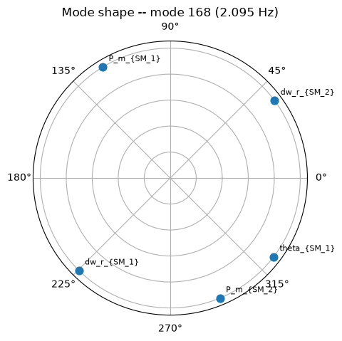
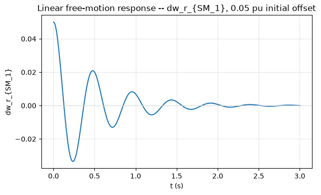
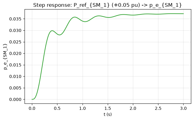
eigenvalue_sensitivity(modal, A, mode, n_top=8) — how sensitive one mode’s own eigenvalue is to each structurally-nonzero entry of \(A\) (Kundur’s own sensitivity result, \(\partial\lambda_i/\partial A_{kj} = w_i[k]v_i[j]\)).
mode_shape(modal, mode, n_top=5) — relative phase between a mode’s own top participating states.
free_response(modal, perturb_index, offset, t) — closed-form response to an initial-condition perturbation.
step_response(system, input_name, output_name, amplitude, t) — MIMO step response between one chosen input/output pair.

All four need one specific mode to look at – picking the mode with the highest raw participation from dw_r_ (a synchronous machine’s own speed deviation) finds the network’s electromechanical swing mode directly, rather than accidentally landing on the network’s own structurally-near-zero reference-angle mode (see the eigenvalue-map cell above and docs/sphinx/modules/stability.md’s “theta problem” note – that mode is real but isn’t an oscillation to look at with any of the four functions below).

from g2elin_core.modal.toolbox import eigenvalue_sensitivity, mode_shape, free_response, step_response

summary = modal.summary_table()
swing = summary[summary["state1"].str.contains("dw_r_")].sort_values("damping_pct").iloc[0]
mode_idx = int(swing["mode"])
print(f"Swing mode: #{mode_idx}, {swing['damped_hz']:.3f} Hz, {swing['damping_pct']:.1f}% damping, "
      f"top state: {swing['state1']} ({swing['part1_pct']:.1f}%)")

sens = eigenvalue_sensitivity(modal, system.A, mode_idx, n_top=8)
print(f"\nTop {len(sens.top)} entries A is most sensitive to:")
for entry in sens.top:
    print(f"  d(lambda)/d(A[{entry.row_state}, {entry.col_state}]) = {entry.value:.4f}")

Swing mode: #168, 2.095 Hz, 12.8% damping, top state: dw_r_{SM_1} (28.1%)

Top 8 entries A is most sensitive to:
  d(lambda)/d(A[dw_r_{SM_1}, P_m_{SM_1}]) = 25.3649
  d(lambda)/d(A[dw_r_{SM_2}, P_m_{SM_2}]) = 14.5631
  d(lambda)/d(A[dw_r_{SM_2}, i_gd_{SM_2}]) = 11.3657
  d(lambda)/d(A[dw_r_{SM_1}, psi_d_{SM_1}]) = 5.9861
  d(lambda)/d(A[dw_r_{SM_1}, psi_q_{SM_1}]) = 4.1213
  d(lambda)/d(A[dw_r_{SM_1}, psi_1d_{SM_1}]) = 3.3568
  d(lambda)/d(A[dw_r_{SM_2}, psi_d_{SM_2}]) = 3.1249
  d(lambda)/d(A[dw_r_{SM_1}, psi_2q_{SM_1}]) = 3.1057

shape = mode_shape(modal, mode_idx, n_top=5)

fig, ax = plt.subplots(figsize=(5, 5), subplot_kw={"projection": "polar"})
angles = np.radians(shape.angles_deg)
ax.scatter(angles, [1] * len(angles), s=60, color="tab:blue", zorder=3)
for a, name in zip(angles, shape.states):
    ax.annotate(name, (a, 1), textcoords="offset points", xytext=(6, 6), fontsize=8)
ax.set_yticklabels([])
ax.set_title(f"Mode shape -- mode {mode_idx} ({swing['damped_hz']:.3f} Hz)")
plt.show()

../_images/c090722d60694d26216e2569d2d758084cf125402933e9ccdcc2f70022588e8e.png

perturb_name = swing["state1"]
perturb_idx = system.state_names.index(perturb_name)
t = np.linspace(0, 3.0, 400)
x_lin = free_response(modal, perturb_idx, offset=0.05, t=t)

fig, ax = plt.subplots(figsize=(7, 4))
ax.plot(t, x_lin[perturb_idx, :], color="tab:blue")
ax.axhline(0, color="0.85", lw=0.8)
ax.set_xlabel("t (s)"); ax.set_ylabel(perturb_name)
ax.set_title(f"Linear free-motion response -- {perturb_name}, 0.05 pu initial offset")
ax.grid(True, alpha=0.3)
plt.show()

../_images/46458ef5e0a5d67e8dd453fc4eac320211a8842c793f6279382883d20c9d5881.png

sm_input = next(n for n in system.input_names if n.startswith("P_ref_{SM"))
sm_output = next(n for n in system.output_names if n.startswith("p_e_{SM"))
y_step = step_response(system, sm_input, sm_output, amplitude=0.05, t=t)

fig, ax = plt.subplots(figsize=(7, 4))
ax.plot(t, y_step, color="tab:green")
ax.set_xlabel("t (s)"); ax.set_ylabel(sm_output)
ax.set_title(f"Step response: {sm_input} (+0.05 pu) -> {sm_output}")
ax.grid(True, alpha=0.3)
plt.show()

../_images/4faacbc2b20630428055477890ec62c3b93ec354957baad62e153ca1e0e8fe0e.png

6. Nonlinear EMT simulation — every option

timedomain.emt.simulate() integrates the network’s actual nonlinear differential-algebraic equations (a coupled Newton solve at every timestep) instead of the linearized \(A\) matrix above. Building the model (assembling blocks, no integration yet) is cheap, so it stays unconditional.

Every option simulate() takes, not just the ones this notebook happens to use:

Parameter	Meaning
`t_span`	`(t0, t_final)` — the integration window
`x0`	Initial state; defaults to the model’s own operating point
`u_exo_fn`	`t -> exogenous-input vector` — drives a disturbance by changing a reference over time, instead of (or in addition to) perturbing a state; defaults to holding it fixed
`t_eval`	Explicit sample times to return; defaults to the solver’s own adaptive steps
`method`	`scipy.integrate.solve_ivp`’s integrator — default `"Radau"` (implicit, L-stable — this system’s stiffest modes reach ~\(10^6\)–\(10^7\) rad/s); `"BDF"`/`"LSODA"` are other implicit options, explicit methods (`"RK45"`) aren’t recommended for a system this stiff
`rtol` / `atol`	Relative/absolute integration tolerance
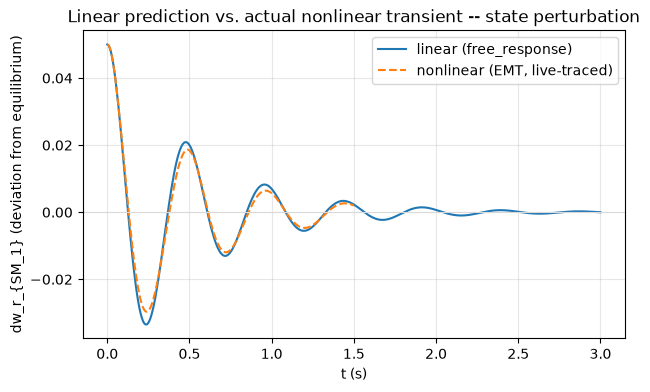
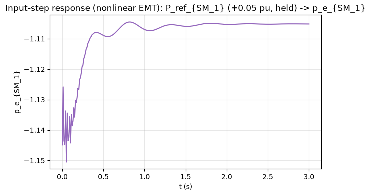
`first_step`	Initial step size hint; a tiny value (e.g. `1e-8`) helps the solver get past the sharp initial algebraic-consistency transient every trajectory starts with

Two demonstrations follow: perturbing a state (an initial-condition offset) and perturbing an input via u_exo_fn (a permanent step in an exogenous reference, held from \(t=0\)) — the same perturb_kind choice the web UI’s EMT tab exposes.

from g2elin_core.timedomain.emt import build_nonlinear_network, simulate

model = build_nonlinear_network(net, pf)
print(f"nonlinear model: {len(model.state_names)} states, {len(model.input_names)} inputs, "
      f"{len(model.output_names)} outputs")

nonlinear model: 176 states, 22 inputs, 28 outputs

6a. Perturbing a state — traced live, step by step

simulate() (Section 6’s own t_eval/method/… table above) is a one-shot call: scipy.integrate.solve_ivp runs straight through to completion and only returns the finished trajectory, with no way to watch it happen. Getting a genuinely live trace means bypassing that convenience wrapper and driving scipy.integrate.Radau’s own low-level stepper object directly — the same algorithm, called one step at a time instead of all at once, redrawing an external plot window after each step.

This still isn’t a literal fixed timestep — Radau is an adaptive implicit method; there is no mode where it takes uniformly-sized steps. max_step below is the honest equivalent of “a specified fixed step value” for an adaptive solver: it caps how large any single step (and so any single redraw) is allowed to get, without forcing every step to actually be that size — the solver can still take smaller steps than max_step where the dynamics demand it (e.g. through the sharp initial transient), it just can never take a larger one.

The live window itself won’t appear in this saved notebook. Unlike an inline plt.show(), an external window isn’t something nbconvert --execute’s headless run (or the Sphinx-embedded copy of this notebook) can capture — Part 2 below re-plots the same result as a normal embedded static figure once the live run finishes, so the comparison is still visible either way. The live window only shows up if you run this cell yourself, in a live kernel.

if RUN_EMT_SECTION:
    import scipy.integrate

    x0 = model.initial_state()
    xp = x0.copy()
    xp[perturb_idx] += 0.05

    t_final = 1.5
    max_step = 0.01  # caps the adaptive solver's own step -- see the markdown above

    # The same warm-started coupled-algebraic-solve pattern simulate() itself uses
    # internally (g2elin_core/timedomain/emt.py) -- replicated by hand here because
    # solve_ivp() can't yield control back between steps; the OOP stepper can.
    u_exo_default = model.default_u_exo()
    z_guess, u_guess = model.initial_algebraic_guess()
    cache = {"z": z_guess, "u": u_guess}

    def rhs_fn(t, x):
        xdot, z_sol, u_sol = model.rhs(x, u_exo_default, cache["z"], cache["u"])
        cache["z"], cache["u"] = z_sol, u_sol
        return xdot

    stepper = scipy.integrate.Radau(
        rhs_fn, 0.0, xp, t_final, max_step=max_step, rtol=1e-4, atol=1e-6, first_step=1e-8,
    )

    # Switch to an external interactive window for this one cell only -- switched
    # back to the notebook's own inline backend right after, so every later cell
    # keeps producing normal embedded static plots.
    get_ipython().run_line_magic("matplotlib", "tk")
    plt.ion()
    fig, ax = plt.subplots(figsize=(7, 4))
    line, = ax.plot([], [], color="tab:orange")
    ax.set_xlim(0, t_final)
    ax.set_xlabel("t (s)"); ax.set_ylabel(f"{perturb_name} (deviation from equilibrium)")
    ax.set_title("Live nonlinear EMT trace")
    ax.grid(True, alpha=0.3)
    fig.canvas.manager.set_window_title("EMT simulation -- live")
    fig.show()

    t_hist = [0.0]
    x_hist = [float(xp[perturb_idx] - x0[perturb_idx])]

    while stepper.status == "running":
        stepper.step()
        t_hist.append(stepper.t)
        x_hist.append(float(stepper.y[perturb_idx] - x0[perturb_idx]))
        line.set_data(t_hist, x_hist)
        ax.set_ylim(min(x_hist) - 0.005, max(x_hist) + 0.005)
        fig.canvas.draw()
        fig.canvas.flush_events()

    if stepper.status == "failed":
        raise RuntimeError(f"live EMT integration failed at t={stepper.t:.4f}")

    plt.ioff()
    plt.close(fig)
    get_ipython().run_line_magic("matplotlib", "inline")

    t_eval = np.array(t_hist)
    nonlinear_trace = np.array(x_hist)
    print(f"live integration finished: {len(t_hist)} steps, t_final={t_hist[-1]:.4f}")

live integration finished: 2052 steps, t_final=1.5000

Now the ordinary static comparison, exactly like the rest of this notebook’s own plots (and what actually gets saved/rendered): the live run’s own result overlaid against Section 5’s closed-form linear prediction.

if RUN_EMT_SECTION:
    fig, ax = plt.subplots(figsize=(7, 4))
    ax.plot(t, x_lin[perturb_idx, :], color="tab:blue", label="linear (free_response)")
    ax.plot(t_eval, nonlinear_trace, color="tab:orange", ls="--", label="nonlinear (EMT, live-traced)")
    ax.axhline(0, color="0.85", lw=0.8)
    ax.set_xlabel("t (s)"); ax.set_ylabel(f"{perturb_name} (deviation from equilibrium)")
    ax.set_title("Linear prediction vs. actual nonlinear transient -- state perturbation")
    ax.legend()
    ax.grid(True, alpha=0.3)
    plt.show()

../_images/66102575bea966222fa47e6d96da425528fcd2b15c595c87b83c50f8f99b8ae4.png

6b. Perturbing an input, via `u_exo_fn`

A state perturbation moves the starting point away from equilibrium but leaves every reference (P_ref, Q_ref, …) exactly where it was; an input perturbation instead moves the equilibrium itself — the system starts at its own operating point and is then asked to track a new one.

if RUN_EMT_SECTION:
    input_idx = model.input_names.index(sm_input)
    perturbed_u_exo = model.default_u_exo()
    perturbed_u_exo[input_idx] += 0.05
    u_exo_fn = lambda t: perturbed_u_exo  # held constant at the stepped value for all t -- noqa: E731

    t_eval_u = np.linspace(0, 3.0, 300)
    sim_u = simulate(
        model, (0.0, 3.0), u_exo_fn=u_exo_fn, t_eval=t_eval_u,
        method="Radau", rtol=1e-4, atol=1e-6, first_step=1e-8,
    )
    # p_e is an output, not a state -- solve_ivp only returns state
    # trajectories, so recover it from the already-integrated samples.
    _, outputs_u = model.recover_inputs_and_outputs(sim_u.t, sim_u.x, u_exo_fn=u_exo_fn)

    fig, ax = plt.subplots(figsize=(7, 4))
    ax.plot(t_eval_u, outputs_u[sm_output], color="tab:purple")
    ax.set_xlabel("t (s)"); ax.set_ylabel(sm_output)
    ax.set_title(f"Input-step response (nonlinear EMT): {sm_input} (+0.05 pu, held) -> {sm_output}")
    ax.grid(True, alpha=0.3)
    plt.show()

../_images/28143a551a6d40de9425a168668ba3d7a351419f9c29c01856f757e7afc29637.png

7. Layer 1 — what pydantic rejects outright

Network’s own validators run every time you construct one, so these two mistakes never even produce an object to inspect – the exception is immediate, at Network(...) itself.

import copy
from pydantic import ValidationError

bad = net.model_dump()
bad["lines"][0]["to_bus"] = 9999  # references a bus that doesn't exist

try:
    Network(**bad)
except ValidationError as e:
    print("dangling bus reference ->", str(e).splitlines()[0])

dangling bus reference -> 1 validation error for Network

bad = net.model_dump()
bad["der_units"][0]["bus_type"] = "pv"  # was the slack -- now zero slack units

try:
    Network(**bad)
except ValidationError as e:
    print("zero slack units ->", str(e).splitlines()[0])

zero slack units -> 1 validation error for Network

8. Layer 2 — what `validate_network()` catches

These are all perfectly constructible Network objects (every bus reference resolves, there’s exactly one slack) – pydantic has nothing to say about them. They’re still wrong, and would otherwise surface as a bare crash deep inside operating_point.py or interconnect/ network_assembly.py instead of a clear message. validate_network() is what this project uses to catch them proactively – and it reports every issue in one pass, not just the first one it trips over.

def show(label, issues):
    print(f"--- {label} " + "-" * (40 - len(label)))
    if not issues:
        print("  (no issues)")
    for i in issues:
        print(f"  [{i.severity}] {i.message}")
    print()

# A DER's transformer landing on another DER's own bus, plus a line wired
# directly onto a DER's own bus -- two independent mistakes, both caught
# in the same pass.
broken = net.model_copy(deep=True)
d0, d1 = broken.der_units[0], broken.der_units[1]
for tr in broken.transformers:
    if tr.lv_bus == d1.bus:
        tr.hv_bus = d0.bus  # should be a grid bus, not d0's own bus
broken.lines.append(Line(from_bus=d0.bus, to_bus=d1.bus, r_pu=0.01, x_pu=0.1, b_pu=0.0))

show("DER wired to DER (2 mistakes)", validate_network(broken))

--- DER wired to DER (2 mistakes) -----------
  [error] a line's from_bus (bus 16) is DER unit id=1 (sm)'s own bus -- a DER's own bus may only be reached through its own transformer, never a line directly
  [error] a line's to_bus (bus 17) is DER unit id=2 (sm)'s own bus -- a DER's own bus may only be reached through its own transformer, never a line directly
  [error] DER unit id=2 (sm)'s own transformer connects directly to DER unit id=1 (sm)'s bus (16) instead of a plain grid bus

# Two DER units sharing one bus.
broken = net.model_copy(deep=True)
broken.der_units[1].bus = broken.der_units[0].bus

show("two DERs sharing a bus", validate_network(broken))

--- two DERs sharing a bus ------------------
  [error] DER units id=2 and id=1 are both on bus 16 -- each DER unit needs its own private bus

# A load placed on a DER's own private bus instead of its p_cons_mw field.
broken = net.model_copy(deep=True)
broken.loads.append(Load(bus=broken.der_units[0].bus, p_mw=5.0, q_mvar=1.0, name="stray"))

show("load on a DER's own bus", validate_network(broken))

--- load on a DER's own bus -----------------
  [error] load #11 sits on bus 16, DER unit id=1 (sm)'s own bus -- a DER's own local consumption belongs on the unit itself (its p_cons_mw/q_cons_mvar fields), not as a separate Load on its private bus

# Disconnecting the network: drop every line/transformer touching the
# last grid bus's "far side" of the tree by cutting one line and not
# reconnecting it -- here, brute-force: remove all lines entirely.
broken = net.model_copy(deep=True)
broken.lines = []

show("disconnected network (no lines left)", validate_network(broken))

--- disconnected network (no lines left) ----
  [error] the network isn't fully connected (15 separate groups of buses, sizes [2, 2, 2, 2, 2, 2, 1, 1, 1, 1, 1, 1, 1, 1, 1]) -- every bus must be reachable from the slack through lines/transformers

# An unsupported slack type -- a GFM slack still powers flow fine, so this
# is a *warning*, not an error: "ok" stays True, but the affected
# capabilities are called out explicitly.
broken = net.model_copy(deep=True)
broken.der_units[0].unit_type = UnitType.GFM
broken.der_units[0].controller = GfmController.DROOP
broken.der_units[0].xd_pu = None

issues = validate_network(broken)
print("ok:", not any(i.severity == "error" for i in issues))
show("gfm slack (warning, not error)", issues)

ok: True
--- gfm slack (warning, not error) ----------
  [warning] the slack unit (id=1) is a gfm, not a synchronous machine or infinite bus -- power flow works, but modal analysis/EMT don't support a gfm slack yet

9. Robustness across many random networks

One clean draw doesn’t prove the builder is correct by construction – running it across many sizes and seeds, validating every single one before touching power flow or modal analysis, does.

records = []
for seed in range(30):
    r = np.random.default_rng(seed)
    n_grid = int(r.integers(15, 26))  # every draw still >= 15 buses, sizes vary
    n = random_network(r, n_grid_buses=n_grid, name=f"random_seed{seed}")
    issues = validate_network(n)
    ok = not any(i.severity == "error" for i in issues)

    pf_converged = n_states = stable = None
    if ok:
        pf_r = run_power_flow(n)
        pf_converged = pf_r.converged
        if pf_converged:
            sys_r = linearize_network(n, pf_r)
            modal_r = analyze(sys_r.A, sys_r.state_names)
            n_states = sys_r.A.shape[0]
            # 1e-6 tolerance, not a strict "< 0" -- see Section 4's own
            # note: every network here has one eigenvalue structurally
            # pinned near 0 (the "theta problem"), not a real instability.
            stable = bool(np.all(modal_r.eigenvalues.real < 1e-6))

    records.append({
        "seed": seed, "n_grid_buses": n_grid,
        "validate_ok": ok, "n_issues": len(issues),
        "pf_converged": pf_converged, "n_states": n_states, "stable": stable,
    })

df = pd.DataFrame(records)
print(f"{df['validate_ok'].sum()}/{len(df)} validated clean, "
      f"{df['pf_converged'].sum()}/{df['validate_ok'].sum()} of those converged in power flow")
df

30/30 validated clean, 30/30 of those converged in power flow

	seed	n_grid_buses	validate_ok	pf_converged	n_states	stable
0	0	24	True	True	224	True
1	1	20	True	True	198	True
2	2	24	True	True	216	True
3	3	23	True	True	214	True
4	4	22	True	True	204	True
5	5	22	True	True	210	True
6	6	19	True	True	196	True
7	7	25	True	True	228	True
8	8	22	True	True	204	True
9	9	19	True	True	198	True
10	10	23	True	True	210	True
11	11	16	True	True	174	True
12	12	21	True	True	202	True
13	13	24	True	True	222	True
14	14	16	True	True	184	True
15	15	25	True	True	220	True
16	16	20	True	True	196	True
17	17	23	True	True	218	True
18	18	24	True	True	220	True
19	19	21	True	True	200	True
20	20	24	True	True	222	True
21	21	18	True	True	188	True
22	22	23	True	True	220	True
23	23	15	True	True	170	True
24	24	19	True	True	194	True
25	25	20	True	True	196	True
26	26	24	True	True	218	True
27	27	15	True	True	166	True
28	28	22	True	True	208	True
29	29	25	True	True	226	True

Good practices to take away

A DER always gets its own private bus, reached through exactly one transformer — never a Line, never shared with another DER, never another transformer’s hv_bus. This one rule drives most of validate_network()’s checks, because it’s the rule a programmatic or drag-and-drop builder is most likely to break by accident.
A DER’s own local consumption is p_cons_mw/q_cons_mvar, not a separate Load on its bus.
Exactly one slack DER, and prefer sm/infinite_bus for it — pydantic enforces “exactly one” unconditionally; validate_network() additionally warns (not blocks) if it’s a type modal/EMT can’t wire up yet.
Keep the graph connected. A random spanning tree is a cheap way to guarantee this by construction rather than checking for it after the fact — and if the topology is meant to be radial specifically (a distribution feeder, not a meshed transmission network), a spanning tree isn’t just convenient, it’s the definition: no edges beyond it.
Give each DER its own connection point. Nothing in the schema requires two DERs to tap different grid buses, but sampling their dispatch buses without replacement (rng.choice(..., replace=False) above) keeps the example topologically realistic and easier to reason about — two generators electrically coincident at the same point is rarely what a real study intends, even though it’s schema-valid.
Validate before you solve. validate_network() is cheap (no power flow needed) and reports every problem at once — call it as a pre-flight check on anything you generate or hand-assemble, the same way the web UI’s network editor calls POST /api/network/validate on every edit, and the same way compute_operating_point() calls it automatically before doing any real work.

See notebooks/tour.ipynb for the same analysis pipeline exercised module-by-module on the hand-written presets, and docs/sphinx/modules/network.md for the full account of both validation layers.

Building a random network from scratch — a tour of Network’s conventions