Worked example: CIGRE islanded, 1 SM + 1 GFM + 1 GFL

Every other page in this documentation explains one module at a time. This page instead follows one preset network — cigre_islanded_1sm_1gfm_1gfl() — all the way through every module, end to end, with real computed results at each step. It’s a companion to the actual notebook it’s built from, rendered here in full — every code cell, every markdown explanation, and every plot, not just the highlights curated onto this page. Every number and figure below was produced by that notebook, not re-derived by hand; open notebooks/cigre_1sm_1gfm_1gfl_walkthrough.ipynb in this checkout directly for the runnable version (see this project’s own README.md for how to launch a Jupyter kernel against its .venv).

Why this preset: it’s the smallest network in this codebase with one of each major DER type — a synchronous machine, a grid-forming converter, and a grid-following converter — on one shared, fully islanded microgrid (no upstream infinite bus to lean on). That makes it the clearest case for comparing three fundamentally different control philosophies side by side, and for asking, concretely: which one is actually holding this microgrid together?

1. The network

CIGRE’s 14-bus MV benchmark feeder (20 kV, f_hz=50, sn_mva=2.5), islanded with its one normally-open tie line (buses 8-12) closed, plus three DER units each on their own new 10 kV terminal bus behind their own step-up transformer:

id	type	role	dispatch bus	own bus	\(V_{set}\) (pu)	\(P_{set}\) (MW)
1	SM	slack	3	15	1.0	1.25 (not fixed — absorbs the rest)
2	GFM (droop)	PV	12	16	1.0	2.5
3	GFL	PQ	9	17	1.0	2.5

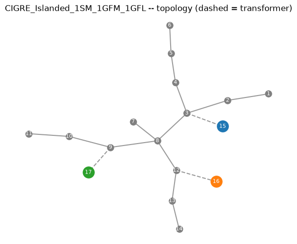
The three DER terminal buses are spread across three different points on the feeder, not clustered — which is exactly what makes the closed tie line load-bearing here: it’s what lets the GFM’s own power actually reach the load buses on the other side of the feeder rather than only serving its own local corner.

2. Power flow

Converges cleanly; every bus sits comfortably within a normal \(\pm5\%\) band even fully islanded — no upstream grid propping up the voltage profile, just the SM’s own AVR and the GFM’s own voltage-droop loop doing that job locally. Reading ext_grid_table(): the SM slack supplies 2.271 MW / 1.469 MVAr — noticeably less than the GFM’s and GFL’s fixed 2.5 MW each — to balance the feeder’s 7.235 MW total load plus losses. That’s the power-flow-level version of “the SM absorbs the mismatch”: it isn’t dispatched to a target, it’s whatever’s left over.

3. Operating point

Three different ways of finding “the angle” a unit’s own dq frame is built around, from the exact same power-flow solution:

• SM: the classical “\(E_q\) behind \(X_q\)” rotor-angle construction — a real physical rotor position, \(\theta_0=-0.906\) rad here (and, being the slack, this is the global reference angle).

• GFM: no rotor to locate — its own frame angle is just its terminal voltage’s angle directly, \(\theta_0=0.0057\) rad.

• GFL: PLL-locked to the terminal voltage the same way, and by construction its own \(v_{eq0}\approx 0\) — a PLL’s entire job is to drive \(v_{eq}\to0\), so the dq frame’s \(d\)-axis ends up aligned with the voltage vector automatically.

See pu_base and operating_point for the full derivation behind each of these.

4. Components, in isolation

Before interconnection, each unit’s own linearization gives its open-loop state count: 19 states for an SM with its default regulators (electrical + mechanical

• AVR + PSS), 15 for the GFM (LCL filter + DC link + droop + voltage/current loops), 14 for the GFL (the same filter/DC-link structure, current-controlled with a PLL instead of self-clocking) — see components — symbolic nonlinear-then-linearized models for exactly what each state is.

5. Interconnection

\(19+15+14=48\) DER states, plus \(2\) states per plain node/line/load — all 14 raw feeder buses, all 13 lines, all 13 loads each contribute their own dynamic state (this project’s DAE formulation wires the network together as coupled ODEs, not a reduced admittance matrix — see interconnect — wiring components into one closed-loop system):

\[ 48 + \underbrace{14\times2}_{\text{nodes}} + \underbrace{13\times2}_{\text{lines}} + \underbrace{13\times2}_{\text{loads}} = 48+28+26+26 = 128 \text{ states total} \]

6. Modal analysis — reading the eigenvalue map correctly

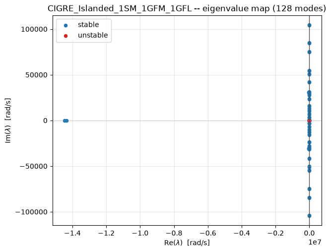
(Plotted at linear scale, unlike the web UI’s symlog-scaled eigenmap — see g2elin_api and the web UI — which is why almost every mode piles up near the imaginary axis here against one far-left cluster of very heavily-damped, very fast modes.)

Sorting by damping percentage surfaces three genuinely different things, and conflating them is the single easiest mistake to make reading this table:

1. Mode #127, 0.000 Hz, \(-100\%\) “damping” — not a real instability. Its real part is \(\sim\!10^{-10}\) rad/s (a centuries-long time constant) and its top participants, theta_{GFM_1}/theta_{SM_1} at almost exactly 50/50, are exactly the “theta problem”: an absolute angle has no restoring force, only angle differences do, so every closed-loop network built by this codebase has exactly one structurally-zero eigenvalue in this direction. The damping_pct formula divides by a near-zero \(|\lambda|\) here, which is why it reports a dramatic-looking \(-100\%\) for what is, physically, a non-event — and why bool(np.all(eigenvalues.real < 0)) reports False for this (and every other) network in this codebase, without that meaning anything is actually unstable.

2. Modes #88/87, \(\approx16{,}639\) Hz, \(0.11\%\) damping — real, but electrical, not mechanical. Dominated by one line’s own current and its endpoint node’s voltage — a fast, lightly-damped-in-percentage (though heavily damped in absolute rad/s) resonance, exactly the kind of “stiff” high-frequency mode timedomain — EMT (nonlinear) time-domain simulation notes the EMT solver has to handle.

3. The mode most people actually mean by “the generator’s own swing” — found by filtering directly for dw_r_{SM_1} participation rather than trusting the raw sort — sits at 2.168 Hz, ~22.0% damping, dominated by dw_r_{SM_1} (40.9%) and P_m_{SM_1} (21.6%). Comfortably stable, and the mode the rest of this page uses.

7. Linear prediction vs. the actual nonlinear transient

Perturbing dw_r_{SM_1} by \(+0.05\) pu and comparing the closed-form linear free_response against a full nonlinear EMT simulation of the same perturbation:

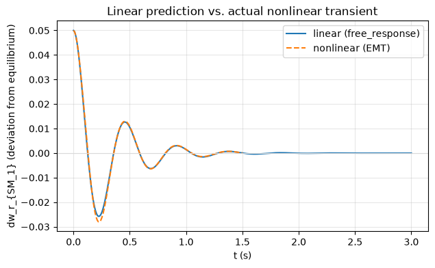
They track closely — a maximum absolute difference of about 0.0024 pu over the full 1.5 s window (under 5% of the initial offset), both decaying to essentially zero by the end, consistent with the swing mode’s own ~22% damping. This is what “small-signal” in “small-signal/ modal analysis” means concretely: a first-order Taylor approximation around the operating point, accurate for small enough deviations and only for small enough deviations — re-running the notebook’s own cell with a much larger offset (0.3-0.5 pu) is a quick way to watch that approximation start to visibly break down.

Note the choice of state matters. The theta-drift mode from Section 6 would have been a poor choice for this comparison: an absolute angle never returns to a fixed operating-point value even at a genuinely stable equilibrium (dtheta/dt = wb*w, integrating continuously), so comparing a nonlinear trajectory’s raw value against a frozen constant for that kind of state diverges by construction — not a sign of instability, just the wrong quantity to compare. dw_r_{SM_1} is a bounded deviation state, which is what makes the comparison above meaningful.

8. Time-series load sweep

Re-solving power flow at 70% / 100% / 130% of the base network’s loads (no dynamics — see timeseries — multi-scenario load flow, no dynamics):

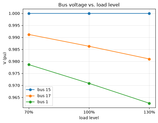
Voltage droops with load everywhere, but not equally: the GFL’s own terminal (bus 17, fixed \(P/Q\) dispatch, no voltage control of its own) moves more with load than the SM’s slack terminal (bus 15, whose AVR is actively holding voltage) — a direct, visible consequence of the same “who’s actually regulating voltage here” question this whole page has been asking.

Summary

Module	What it told us about this network
network	The DER mix, dispatch, and physical layout
powerflow	A feasible, in-range voltage profile; the SM slack supplies ~2.27 MW vs. the GFM/GFL’s fixed 2.5 MW each
operating_point	Three different ways of finding “the angle” — rotor geometry, self-clocked droop, PLL lock
components (isolated)	19/15/14 states for SM/GFM/GFL, and how differently stiff each one’s own open-loop dynamics are
interconnect / pipeline	128 states total: 48 DER + 28 node + 26 line + 26 load
modal	One structurally-zero reference-angle mode (not real instability); the genuine SM swing mode at ~2.2 Hz, ~22% damping
modal.toolbox	Mode shape, closed-form free response, and step response — all from the same eigendecomposition, no extra solve
timedomain (EMT)	The actual nonlinear transient the linearization is only ever a small-signal approximation of — and how good that approximation is here
timeseries	Which bus’s voltage is most exposed to load swings, and why

See notebooks/tour.ipynb for the same modules exercised more briefly across several different presets.